Mesh
- Geological seismic imaging and numerical simulations.
- Levelset extraction.
- Mesh optimization.
- Examples.
Seismic image
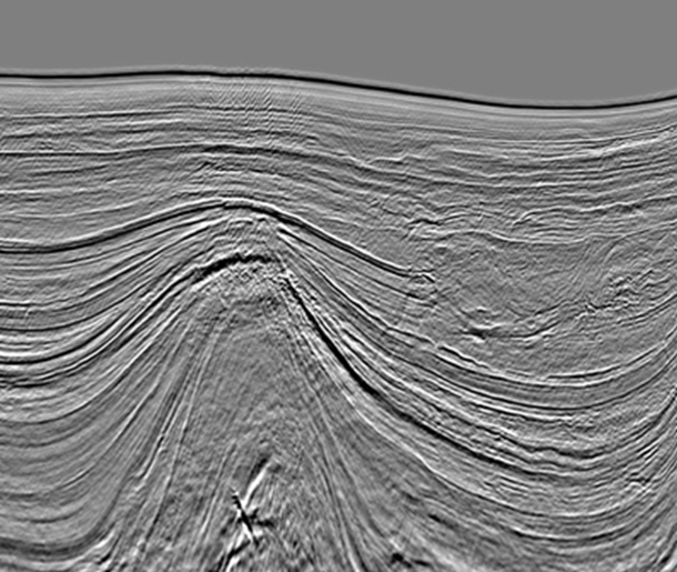
Data collection.
Inversion process.
Interpretation:
Structural model
Processed/interpreted 3D volume
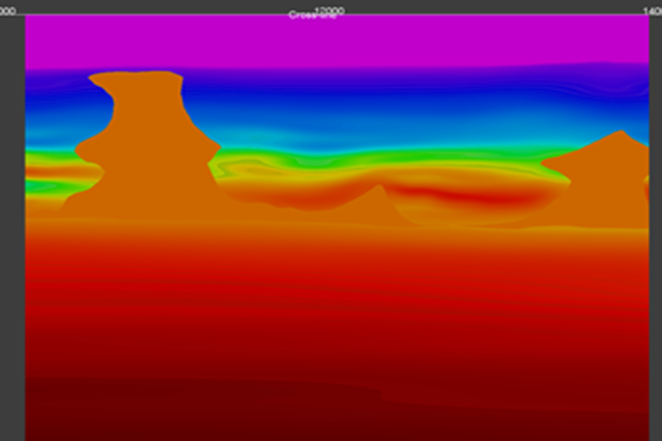
Creating a structural model requires:
Challenges:
Reservoir mesh
The input data is naturally defined on a regular (sugarcube) grid.
There are two general approaches:
Surface triangulations

Automated extractions of:
Advantages:
Surface triangulations
The rectangular grid on which the data exists can be split (non-uniquely) into triangles (2D) or tetrahedrons (3D) and then perform the surface extraction.
Advantages – fast and simple:
Disadvantages:
Basic geometric operations:
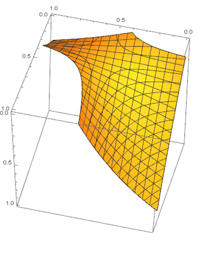
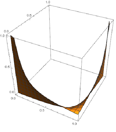
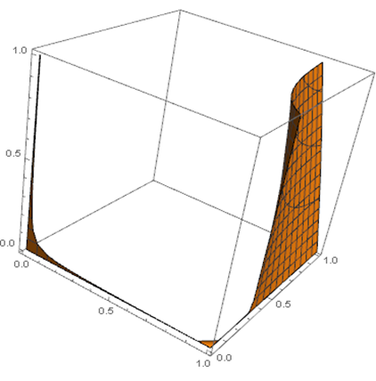
Levelset in cube
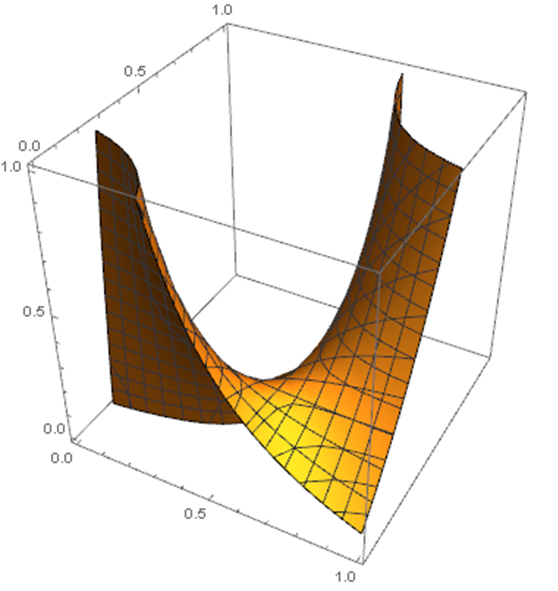
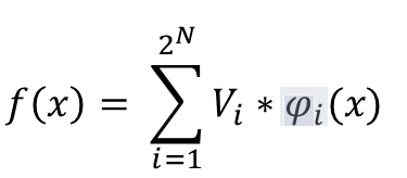
Given 2^𝑁 values in a N-cube we have the usual N-linear interpolation in the N-cube:
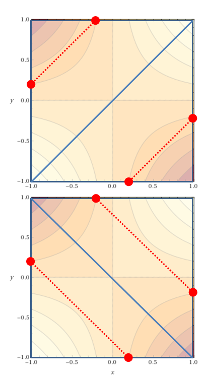
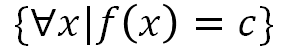
The entire surface is implicitly defined on each cube as follows:
It is conforming across cubes.
Unique representation of the surface.
More accurate topological representation.
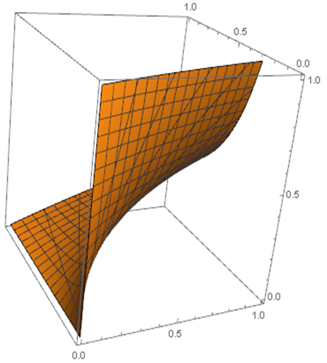
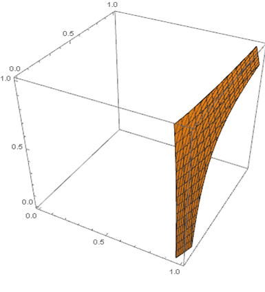
Levelset in cube
Using the bi/tri-linear representation.
Basic geometric operations:
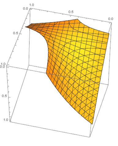
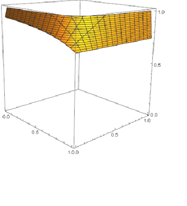
Levelset in cube
Given the definition of the function in a cube, one uses Lagrange multipliers to project in the entire 𝑅^3.
If the projection is outside the cube, use Lagrange multipliers to project on each face (that has a levelset) in the entire 𝑅^2.
If outside of the respective face, check the edges.
Minimize the distance of all candidate points within the cube or on its faces.
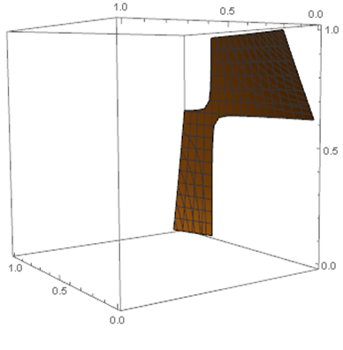
Levelset in cube
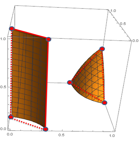
Compute all points on the edges of the hex that are part of the levelset.
Connect points into one or more polygons.
Triangulate the polygon(s).
Collect triangles from all cells into a single surfaces.
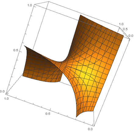
Example 1
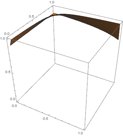
Example 2
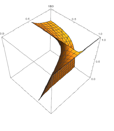
Example 3
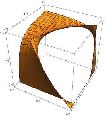
Example 4
Example 5
Example 6
Example 7
Example 8
Example 1
Example 2
Example 3
Example 4
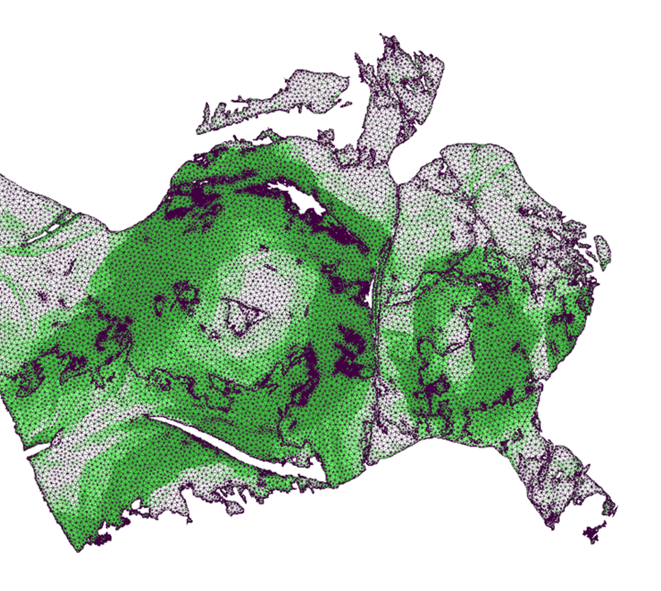
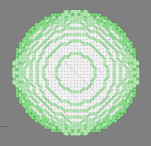
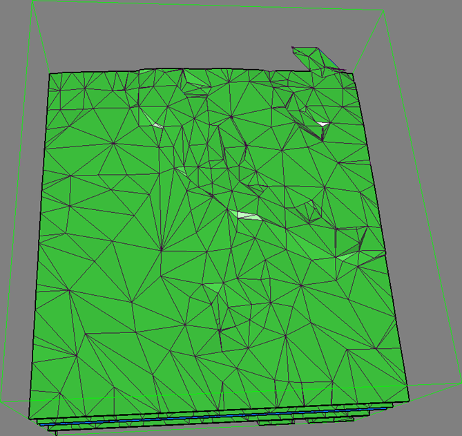
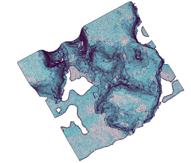
Initial tessellation contains several triangles per original cube.
Quality is typically very bad: small triangles, small angles, etc.
A mesh optimization step is mandatory.
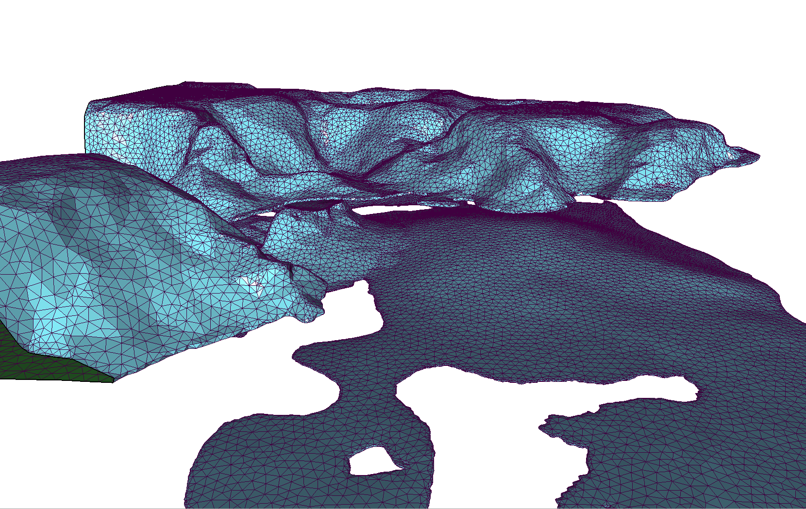
Initial tessellation
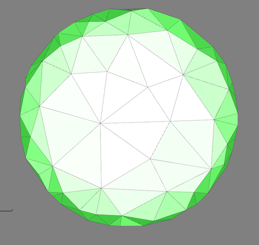
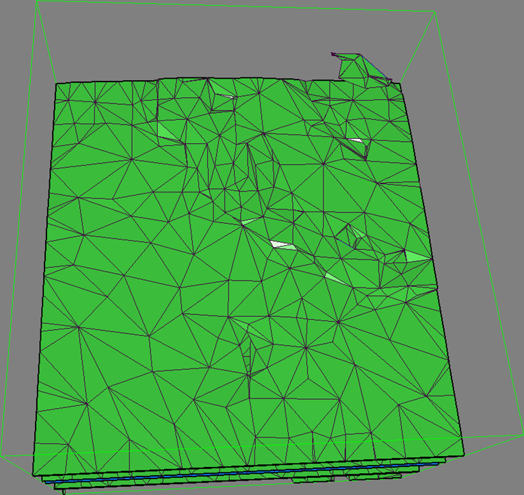
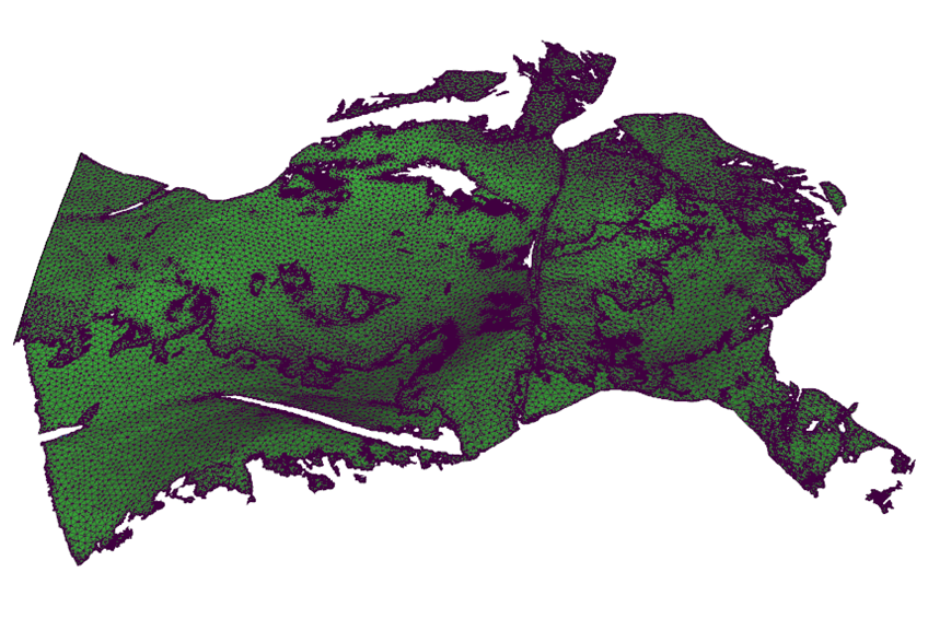
Optimized mesh
Drawing
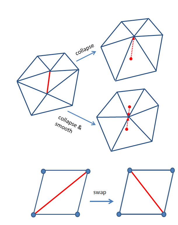
We use a combination of operations on the entire mesh: collapse, swap, refine and smooth.
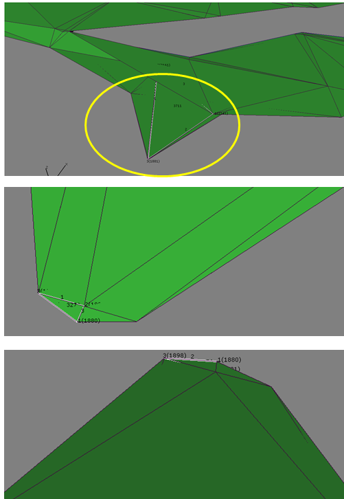
Collapse: the purpose is to eliminate:
Swap:
Smooth:
Refine:
Problems
Approximation parameters:
Mesh quality parameters:
Each operation (Collapse, Swap, Smooth, Refine) evaluates if the new configuration is “better” then the old one.
Criteria for what is “better” are different for each operation.
Greedy optimization does not work!
The definition of “better” local mesh quality is still an active area of research.
Average scheme #1.
Average scheme #2.
Example 1
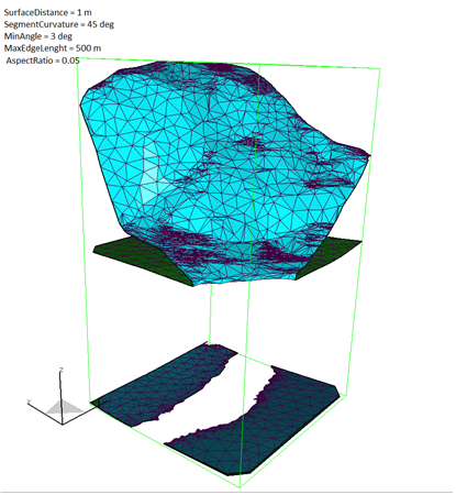
Vertical surface distance: 1 m.
Horizontal surface distance: 20 m.
Min. Angle: 3 deg.
Max Edge Length Restriction: 500 m.
Example 2
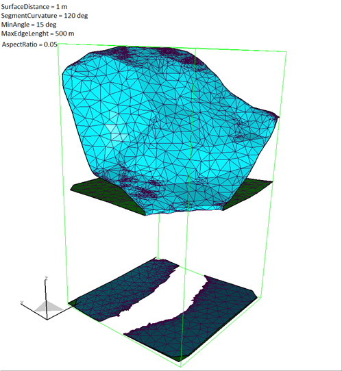
Vertical surface distance: 1 m.
Horizontal surface distance: 20 m.
Min. Angle: 15 deg.
Max Edge Length Restriction: 500 m.
Example 3
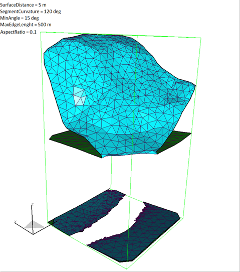
Vertical surface distance: 5 m.
Horizontal surface distance: 50 m.
Min. Angle: 15 deg.
Max Edge Length Restriction: 500 m.
Example 1
Example 2
Example 1
Example 2
Example 3

Mesh
- Levelset extraction based on tri-linear approximation offers a number of advantages.
- An implicit levelset definition can be successfully utilized in mesh optimization schemes.
- An automated workflow has been designed to successfully produce CAD-quality meshes, based on 3D seismic imaging data.
- Tests on medical scans is in progress.